Playgrounds Vs Pubs
This post applies accessibility analysis to compare two types of social amenities: council parks and alcohol vendors - a wider scope than the cheeky alliterative title would suggest. While the accessibility concept is unchanged from the fuel station analysis, the post shows how we can bring together different types (and sources) of spatial data for a richer, and ultimately more insightful analysis.
The motivation for comparing alcohol vendors and parks are two-fold:
- To evaluate local environments by distance to (societally) positive and negative amenities.
- To build a methodology for understanding deprivation as function of the local environment.
The adverse effects of proximity to alcohol are well-documented in research 1. But alcohol isn’t the only societal ill that determines the quality of life in a neighbourhood. There are also effects from other nearby amenities - and likely these amenities heavily interact with each other.
However, we want to start simple. And simple means assuming non-interactivity. So in this post, we’re only looking at the proximity to an alcohol vendor or park proximity as if they were independent from each other i.e. assuming no tradeoffs or conjoined effects between the two.
To accomplish this analysis, we need to manage certain technicalities with obtaining and processing the relevant data. This post covers:
- Getting and processing OpenStreetMap (OSM) ways and nodes into point entities.
- Converting polygon data into points.
- Bringing together the two different spatial sources for comparing accessibility.
- Manipulating the pandana data structure to plot accessibilities within regions of interest.
If bits of the above list don’t make sense, feel free to visit the previous blog post for an introduction to OSM and accessibility analysis. As usual, the code for this post is up as a Jupyter notebook on my github.
Get alcohol vendors from OSM
As highlighted in a previous post, getting data from OSM is quite easy with the Overpass API. For this analysis, ‘shop’, ‘amenity’ and ‘building’ entities with the tags ‘alcohol’, ‘pub’, ‘bar’, ‘beverages’, ‘biergarten’, ‘wine’ and ‘supermarket’ were extracted from OSM. The key difference to the fuel stations analysis is that we have to extend the query to deal with both nodes and ways. For a complete dataset of alcohol vendors, we need two queries since the results are different for nodes and ways.
There is a reasonable probability that we have a small number of duplicates - where the same place has been annotated as both a way and a node. However, for the first pass of the analysis, I’m going to assume that these are negligible. De-duplication will be a part of a more polished, future analysis.
Following the data extraction from OSM, we have to reduce both nodes and ways as POIs (Points of Interest):
- Save the geolocation of nodes
- Process ways as polygons and then reduce to a single geolocation
- Join the two datasets together
Nodes
As we can see in the table below, the nodes dataset is quite simple and the geolocation columns can be easily pulled out.
| id | lat | lon | name | amenity | type |
|---|---|---|---|---|---|
| 4522166458 | -41.328972 | 174.811298 | Cook Strait Bar | bar | node |
| 623879839 | -41.325184 | 174.820872 | The Strathmore Local | pub | node |
| 625080280 | -41.319506 | 174.794358 | Bay 66 | pub | node |
| 4362160389 | -41.318292 | 174.794757 | No Name | No Name | node |
| 627273501 | -41.318117 | 174.794450 | Kilbirnie Tavern | pub | node |
Ways
Unlike the nodes dataset, way data from OSM comes without an explicit geolocation. Instead, it contains a column with a list of node IDs that link to form the way. This means that we can get the multiple geolocations for a way - one for each node in the nodelist. Helpfully, OSM sends such a nodelist so we can extend the ways to a list of nodes. This extended dataset can be reduced by calculating an ‘average’ lattitude and longitude for each way.
| id | lat | lon | name | amenity | type | nodes |
|---|---|---|---|---|---|---|
| 26509771 | NaN | NaN | New World | NaN | way | [290565312, 290565316, 2990208452, 2990208451,… |
| 49396700 | NaN | NaN | Countdown | NaN | way | [627273504, 4699896634, 627273505, 4199712656,… |
| 62153738 | NaN | NaN | Mac’s Brewery | pub | way | [775428527, 775428528, 775428657, 775428658, 2… |
| 62154227 | NaN | NaN | Countdown Johnsonville | NaN | way | [1439843310, 1439843337, 1439843339, 143984333… |
| 133129214 | NaN | NaN | Thistle Inn | bar | way | [1464807182, 1464807184, 1464807179, 146480718… |
The function data_processing.extend_ways_to_node_view() expands the ways data structure into a tall node list with multiple geolocations per way. We can then perform a simple aggregation of a mean lattitude and longitude for each way ID. The mean geolocation is basically the centre of the way (centroid) - assuming of course that the nodes in the way are distriuted evenly!
Alcohol vendors in Wellington
The centroid geolocation for the ways and the point locations for nodes can be plotted on a map. As expected, the Wellington CBD contains the highest density of alcohol vendors.
Quality of alcohol vendor data
The paper by Bright et al. gives an excellent overview of why alcohol research is important - in terms of spatial availability. It also evaluates the use of alcohol vendor data from Open Street Map. Though the analysis was carried out for the UK, we can extrapolate the general principle that data is unlikely to be complete for NZ. Possibly even more so since we’re a smaller country, and OSM has a much greater set of contributers in the UK - owing to the fact that OSM began in the UK.
Alternatives: NZLII
An alternative source of alcohol data to OSM is the New Zealand Legal Information Institute’s database on alcohol licence decsions. The site for Wellington is here. The licence requests for the current year can be examined in detail. Unfortunately, the decisions are uploaded as pdfs.
While text can be extracted from the pdfs, the retreival of information requires a few components:
- Web scraping with bs4 to systematically download all the pdfs of decisions for a given year.
- Loading the pdf as an object with PyPDF2.
- Searching the text with well-constructed regular expressions to get the name of venue and the decision.
- Matching the licence venues to a geolocation. Adding in missing venues to OSM.
While this can actually be done, I’d need some help in crafting the regular expression. The project will consume a lot of time and will require careful thought around when it would be worth scraping the database.
Alternatives: Healthspace
A Google search led me to this page which aggregates alcohol-related data and research for NZ. From there, I navigated to Healthspace, which makes available Statistical Area 2 level alcohol licence data. The data download portal here as xlsx tables. The interface is clunky unfortunately and the latest data is from 2016. Nonetheless, if we want SA2 or larger area unit aggregates, this data is great. I will make a request to see if they have the licence information available at the individual outlet level.
Get parks data from WCC
While we can use OSM to get data of parks in Wellington, we can utilise easily available open government data! There are two sources of park data available from Wellington City Council (WCC):
As of 18 Sept, I’ve only done the analysis on the polygon data of WCC parks and reserves. Repeating the analysis with playgrounds is a sensible option for a future iteration of this analysis as this allows us to focus on how family friendly a particular region is.
While the WCC data can be regarded as a complete and well-maintained dataset, the data format is intrinsically different to OSM. Instead of a list of node IDs, we have a polygon object.
| name_ | address | geometry |
|---|---|---|
| Ex Wellington Bowling Club Land | Tanera Crescent | POLYGON ((174.765237429376 -41.300402529001, 1… |
| Waimapihi Reserve | Holloway Road | POLYGON ((174.755229696891 -41.2989941468547, … |
| Newlands Plunket/Kenmore Street Play Area | 108 Kenmore Street, Horokiwi Road | POLYGON ((174.825350752449 -41.223283485097, 1… |
| Railway Station Reserve, Bunny Street | Bunny Street | POLYGON ((174.780368233065 -41.2795407305749, … |
| Seatoun Wharf and Boatsheds | Marine Parade | (POLYGON ((174.829013038144 -41.3179656818365,… |
Polygons to POIs
Polygons are special spatial (oh homophonic joy!) data structures that can be manipulated with dedicated spatial software, e.g. the suite of GIS (Geographic Information Systems) like ESRI, ARCGis etc. Hardly one to be left out, Python also provides a suite for spatial data management and manipulation. Enter Geopandas. This library extends dataframes to spatial dataframes. Some of the extensions include methods that operate on spatial data formats. Like polygons. With these methods, it’s very easy to convert a polygon to a centroid - as easy as df[‘polygon_column’].centroid. None of the rigamarole that we went through in the previous section!
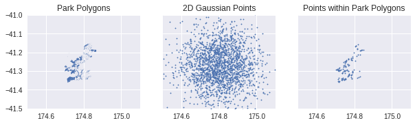
Unfortunately, generating a centroid for a park is not sufficient for accessibility analysis. Some parks are massive and a centroid is not really representative of distance to the park from a nearby street. What we need are several evenly distributed points within the park. With the power of geopandas, this is actually pretty easy to do.
The concept of generating many random but evenly spaced points within a park is simple: we basically superimpose a 2D Gaussian distribution of random coordinates over the park polygons. The joined dataset is now a set of coordinates constrained by the shape of the parks. The illustrative figure shows how the park polygons become a collection of points constrained by the polygon boundaries.
Visualising parks as POIs
We can visualise the distribution of these points in an interactive map. The density of points isn’t high but can be easily increased by altering the parameters of the Gaussian random sampling. I used the plots in the above figure for qualitative checks - that the Wellington park geography was within the ~1 $\sigma$ region of the random points. I can always go back and either increase the number of samples, or change the scale parameter to cover a greater coordinate space.
Accessibility analysis
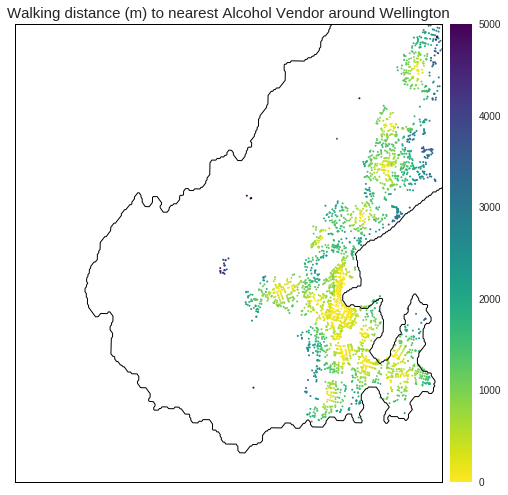
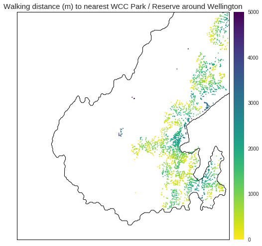
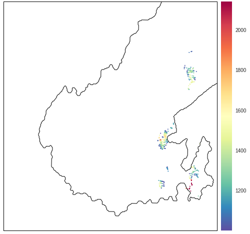
We now have alcohol vendors and parks described by discrete POIs and ready for calculating accessibility. Like the previous series, accessibility is calculated as the driving distance (meters) from each street grid point (also referred to as nodes) to the nearest POI. This driving distance is visualised as a heatmap.
Accessibility analyis made very accessible (pun intended!) by the Python package Pandana. Technical details are described in an earlier post.
Spatial distribution of playgrounds vs. pubs
The accessibility heatmaps illustrate that both parks and alcohol vendors are well distributed (focus on the distribution of the yellow) but there are definite hot spots for both. For example, Wellington CBD is closer to alcohol vendors. This is obvious and easy to pick out from the heatmap. However, there are other non-obvious hotspots of alcohol vendots that are harder to perceive.
 |
 |
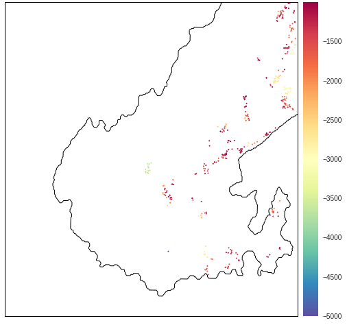
One way to see the relative closeness of an alcohol vendor compared to a park is with a differential accessibility map. Here, we simply take the difference between the distance to the nearest alcohol vendor and park at every street grid point. Positive values indicate greater closeness to an alchol vendor while a negative value means a park is closer. I’ve thresholded the map so that only the street grid points that are closest / furthest away from an alcohol vendor are seen.
These maps now start to show some interesting things (other than the obvious CBD proximity to alcohol!):
- The western part of the Miramar peninsula is much closer to alcohol - though part of this is bias from the airport industrial area.
- There are also pockets of high alcohol vendor proximity in Island Bay, Johnsonville, Newtown.
- The usual suburban suspects, that ring the city and are close to the town belt, are much closer to parks.
| Furthest from alcohol vendor | Closest to alcohol vendor |
|---|---|
 |
 |
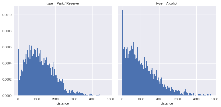
From Spatial to Bayesian
In addition to spatial visualisation, we can also summarise the accessibility values as distributions. Currently, the point distribution of the POIs within the parks may not be ideal so it’s not sensible to read too much into the shape of the accessibility distributions.
Once the POIs methodology is sorted, we have a key advantage of a reduced dataset: the ability to do statistical modelling. My current thoughts include modelling accessibility to a park / alcohol vendor by meshblock with a Bayesian hierarchical model. With such a model, we can pull out differences in accessibility across meshblocks - and a potential extension to the SA2 (loosely corresponding to suburb units). The aim of this analysis would be to see if there are any meshblocks (or SA2s) with higher than average accessibility to a park.