R For Geospatial

Summary

The first part of a proposed three part series on tools for geospatial analysis in the transport domain. This review details functionality of three key R packages: stplanr, dodgr and tidytransit. Because of the transport focus, other notable packages for geospatial analysis, like sf, are not covered in this particular review series.

Introduction

The battle of R vs. Python for data science is a constantly raging one for practitioners. Many choose their side and stick to it vehemently but others, like me, flit from one side to another using the Whatever is best for problem at hand excuse. I say ‘excuse’ because sometimes it feels like I’m simply biding my time for a clear winner to emerge. At other times, ‘excuse’ is the wrong word because I do truly feel like each has their strengths and cutting-edge tools and packages are not developed simultaneously in both ecosystems.

My first port of call is usually Python, even though I think dplyr (and the tidyverse) is far better than pandas. Python is an easy start because:

• The syntax is easy
• Verbose loops for lazy and quick coding aren’t poorly performant (unlike R!)
• You don’t have to remember too many onliners / idioms

Reason (3) is touted as a major scoring point for R afficianados but when data science work spans across many domains, the suite of necessary packages (and idioms) grows substantially - a real travail for those of us with poor memory.

True to my preference my previous forays into analysing transport, specifically walking, have used the Python suite of geospatial and analysis packages e.g. geopandas, osmnx, pandana, pandas, numpy, seaborn and pystan. However, in less than a week, I’ll be transitioning to a new employer whose data science will be driven by R. This imminent move has prompted a self-learning spike culminating in this literature review of R packages that support spatial analyses (particularly pertaining to transport).

I hope to split this review into three main parts; starting with a focus on R tools, exploring the Python side and wrapping up with a comparison of the two ecosystems. The reason for this triple pronged approach links back to the introduction citing the asymmetry in functionality available in R vs. Python. I know there are other on the fence Data Scientists so I’m hopeful that this review will save some time and effort in scouting out the best tool / ecosystem for geospatial analyses.

Enter Robin Lovelace

A quick Google search will reveal that the lynchpin of knowledge, innovative work, and package development in the R geospatial world is Dr. Robin Lovelace. He’s an active developer of stplanr, a key transport analysis package, and part of several other open data and open transport initiatives. For example, Propensity to Cycle Tool (PCT), Active Transport Futures and a recent open textbook Geocomputation with R.

Singling Robin out is not meant to downplay the contributions of countless others but that he plays quite a central role in opening up the R geospatial world to a relative newbie. For example, much of this particular post is inspired by Robin’s talk at UseR2019.

The R geospatial movement that Robin is part of looks very familiar to the explosion of concerted activity that accompanied ggplot2 and dplyr. Now, these pioneering packages form a core suite of R packages for Data Science known as the tidyverse. A similar vision appears to be in place for geospatial analyses with core packages like stplanr, dodgr and tidytransit (described in the next section) slotting together nicely.

Modular packages of the tidyverse
Image from the tidyverse website

The limited package tour

Or perhaps Caveat Lector (Reader Beware) - a dramatic way of noting that this review is not intended to be a comprehensive one. Inspired by Robin’s presentation, the following core packages are described in some detail: dodgr, tidytransit and stplanr. While this set of packages is not comprehensive, they cover considerable ground in terms of geospatial analyses:

• Wrangling geospatial data formats
  • Spatial primitives
  • Origin-Destination data
  • Street networks
  • GTFS
• Calculations and aggregations on spatial objects
  • Network analysis algorithms applied to street networks
  • Routing along the street network with graph algorithms or API calls
  • Aggregating geospatial street network metadata including spatial flows

At the end, I include a couple of other packages, gtfs-router and moveability, that are interesting and useful though they’re not described in much detail.

stplanr

An acronynm for Sustainable Transport PLANning in R, stplanr is a transport planning utility developed by Robin Lovelace. The package has several unique value propositions which can be split into three categories: data, functions and analyses.

Data

According to the stplanr paper, paraphrased below, the core functions are structured around 3 common types of spatial transport data:

• Origin-destination (OD) data: the number of entities travelling between origin-destination pairs. This type of data is not explicitly spatial (OD datasets are usually represented as data frames) but represents movement over space between points in geographical space.
• Line data: one dimensional linear features on the surface of the Earth. These are typically stored as a SpatialLinesDataFrame.
• Route data: a special type of lines which have been allocated to the transport network.

Functions

The functions provided in the stplanr package manipulate the three spatial transport data types described above.

• Downloading and cleaning transport datasets
• Creating geographic ‘desire lines’ OD data
• Creating routes via the SpatialLinesNetwork class or API calls to services such as CycleStreets.net
• Calculating route segment attributes such as bearing and aggregate flow

Evaluating routes for different transport modes is a key functionality of the package. The package provides oneliner functions to get routing information from several APIs. In addition, there is a handy batch processing function that can manage many routing API calls.

Analyses: Transport modelling

stplanr is intended as a complementary tool to the more intensive transport modelling packages like SUMO. At a basic level, transport modelling starts with the Four Stage Transport Model.

Four Stage transportation model
Original figure reference hard to trace

• Stage 1: Trips are estimated with available data including demographics and availability of jobs.
• Stage 2: Trips are then distributed according to a mathematical decay function - where closer trips are more probable than ones further away.
• Stage 3: Trips are split by mode type - at a trivial level, deciding what fraction will be done by car vs. other modes like public transport, walking etc.
• Stage 4: Origin-Destination flows are assigned to the street network.

stplanr enables most of the 4 stages though it’s still filling out some features especially when it comes to distributing trips. However, with OD data from surveys, the transport model can be analysed to the final stage since the Trip Distribution is replaced by explicit information of flow.

LHS: Origin-Destination flows overlaid on street network. RHS: aggregation of flows onto the street network itself (Stage 4 of transport model)
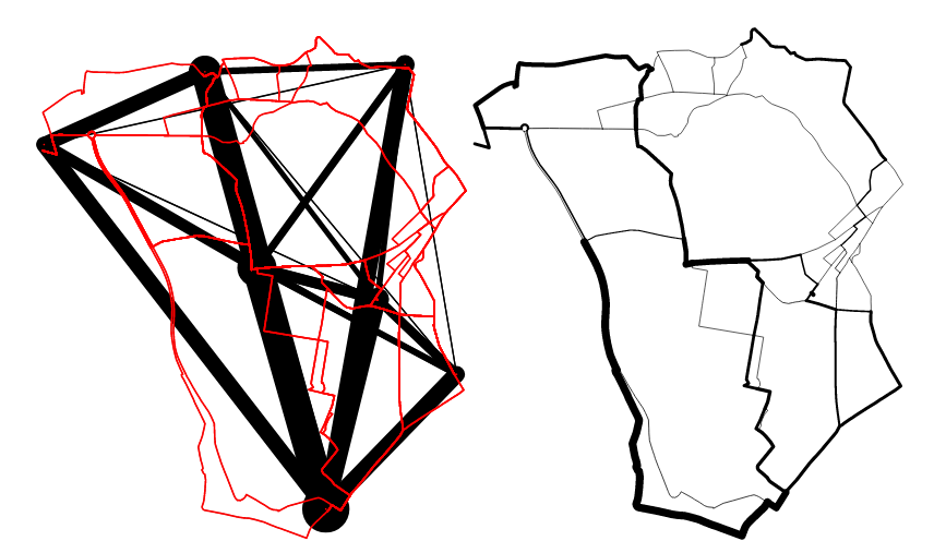Image from the stplanr paper in The R Journal

Analyses: Transport mode split in spatial flows

Transport is a complex beast with multi-modal travel being quite common. stplanr enables modal analyses by separating flow contributions. The propensity to cycle and health impacts of cycling to school on children in the UK have been carried out with stplanr.

Small multiples view of spatial flow for different transport modes
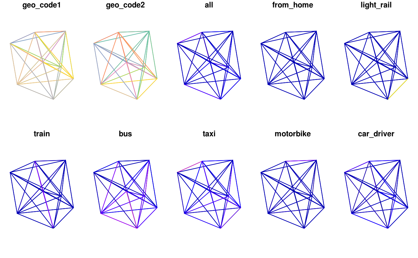Image from the stplanr introduction

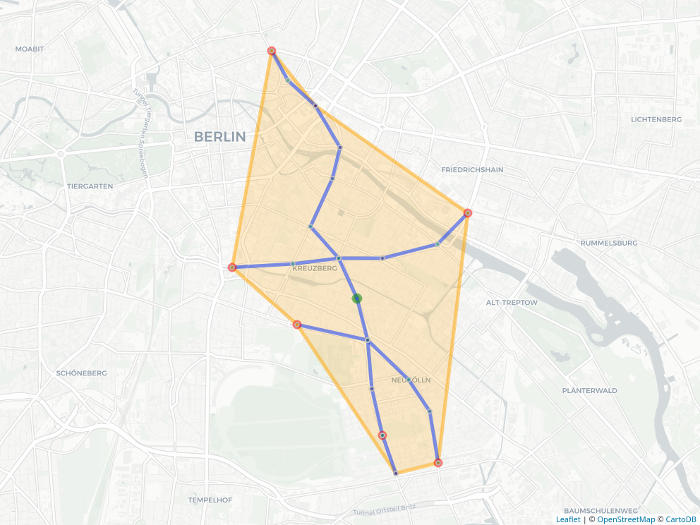
Analyses: Catchment areas

While catchment areas are not a highlighted feature of the package, they are an important part of transport planning - from accessibility of bus stops to cycleways. stplanr can aggregate catchment areas for complex entities like disconnected cycleways.

Catchment areas of cycleway stretches (green lines) specified by Euclidean distance (red) vs. traversing the street network (blue)
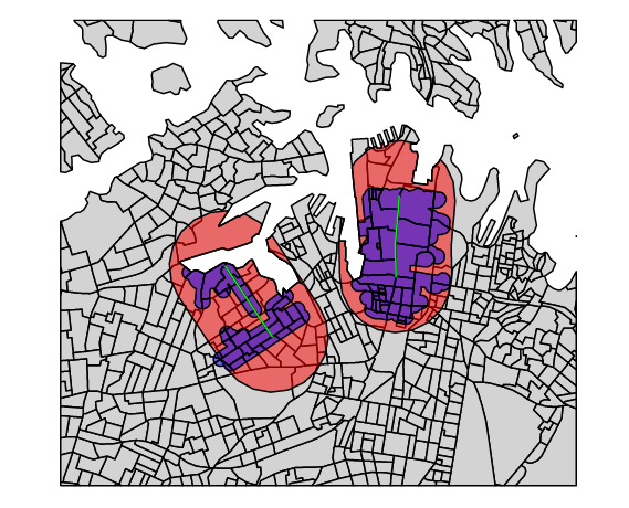Image from the stplanr paper in The R Journal

dodgr

An acronym for Distances On Directed Graphs in R. dodgr can perform graph analysis with street networks and extends graph data aggregation to spatial flow data. A recent publication by the package author, Mark Padgham, states the core functionality to be extensive, customisable and efficient flow aggregation.

The dodgr package has been intentionally developed to be adaptable to any type of network, with a particular focus on flow aggregation through street networks.

A dual directed graph. Grey lines could indicated bicycle flows and black lines can be car flows between points on the street network
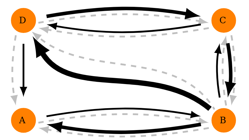Image from the dodgr CRAN vignette page.

According to the package site, dodgr has a fourfold unique proposition:

• Accurate calculation of distances on street networks
• Specifically designed for many-to-many routing
• Routines to aggregate flows throughout a network
• Highly realistic and fully-customisable profiles for routing through street networks with various modes of transport, and using either distance- or time-based routing

dodgr is a highly customisable package for aggregating metrics along a street network - much more so than stplanr. I suspect that large calculations (e.g. an entire city’s street network) of travel times by different modes (car, bus, cycle etc.) might be better done with this package. One benchmark given for dodgr is 4s for 1 Million pairwise flow aggregations. However, since there is no explicit comparison to another package, we’ll have to trust the author’s claim.

Flows from street segmnents can be easily aggregated and merged and then used to visualise and analyse bottlenecks in road networks. For example, Nur-Sultan road network in the figure below. From my own interests of trying to understand bottlenecks in non-grid cities (like Wellington, New Zealand), this feature holds the greatest appeal and potential for interesting analyses.

Aggregated flows of 1 Million journeys in Astana (Nur-Sultan), Kazakhstan
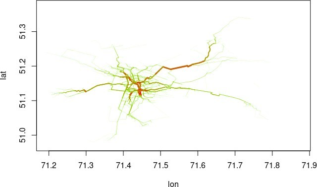Image from a recent publication by the package author

tidytransit

tidytransit can map transit stops and routes, calculate transit frequencies, and validate transit feeds by reading the General Transit Feed Specification (GTFS) into tidyverse and sf dataframes.

GTFS data are quite large and verbose. To ease understanding, tidytransit can do some nifty visualisations - especially from route timetables.

Frequency of services departing from Time Square
Image from tidytransit timetable vignette

The package can also do some insightful spatial aggregations along routes. The underlying dataframes and spatial objects would allow GTFS to be part of bigger analyses in concert with other geospatial packages. For example, integration with stplanr for catchment analysis of bus routes.

Different aggregations of public transport data
Image from tidytransit frequency vignette

gtfs-router

stplanr and dodgr provide graph and API routing algorithms to traverse street networks. gtfs-router can calculate routes given a GTFS feed. The package also has route isochrone functionality that can complement any catchment area analyses.

Isoschrone tracing stops along route
Image from gtfs-router main vignette

moveability

An experimental analysis suite that does some clever number crunching of movability. An R version of pandana without needing POIs for walkability analysis. Pictures below show walkability calculations of Munster, Germany.

Three different aggregations of moveability
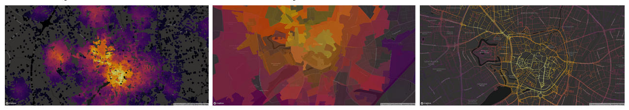Image from moveability Readme